Creating Predictive Maps with R
We now have the tools we need to create predictive maps. The process below can be used to create maps using a wide variety of modeling approaches including linear models, higher-order polynomial models, tree-based models (CART), Generalized Linear Models (GLMs), and Generalized Additive Models (GAMs.). We'll use this approach in the next three labs to create models with different methods.
-
Create a CSV file for modeling. This file should contain your response variables and matching covariate values. There are a variety of ways to create this file but typically you'll:
- Obtain a shapefile of points and measured variables.
- Extract the values from your covariates for your points. In BlueSpray:
- Load the dataset into BlueSpray.
- Right click on the dataset and select "Attributes -> Visible".
- Right click on the right-most column heading and select "Insert Column Right".
- Give the new attribute a good name and make sure the "Data Type" is set to 64-bit floating point.
- When you click "OK", you should see a new attribute column appear.
- Right click on the column heading for the new attribute and select "Extract".
- Select the raster with the count values for the "Attribute".
- Select "Mean" for the "Function" in case the pixels do not line up perfectly.
- When you click OK, you should see the values from the count raster appear in the attribute.
- Now, or later, you can add addtional covariate values to this dataset using the steps above.
- Rght click on the dataset and select "Export To File" and save it to a CSV file.
- Create your model. Use the appropriate modeling methods to create the model.
- Create your predictive data. This is a CSV that represents your entire sample area and contains columns for the x and y coordinate values and your predictor variable values for those points.
- Load a covariate layer such as one from BioClim into BlueSpray.
- To make this process faster, you may want to copy and downsample the raster. After you have the process working, you can then increase the size of the raster to obtain more accurate results.
- To crop the raster:
- Select the marquee tool (dotted box icon)
- Draw a box with the mouse
- Right click on the layer and select "Transforms: General -> Crop Raster"
- In the "Set To" popup, select the AOI (this is the box you created with the maquee).
- Give the new raster a good name such as "Precip_cropped.tif".
- Click OK.
- To downsample the raster:
- Right click on the raster and select "Transforms: General -> Resample"
- Change the "Sample Rate" in the X direction until the size of the raster is about 100 x 100.
- When you click "OK", you should see a raster with large pixels.
- Right click on the raster and select "Transforms: General -> To Points". This step will create a raster with a grid of points where each point contains the value for one pixel in the raster. This is the point dataset we will use for modeling.
- Repeat the steps in section one above to add the values from the other predictor layers into the new grid of points.
- Open the CSV in Excel and change the file's column headers to exactly match the one's you used in R to create the model.
- Predict values for the entire sample area. This step adds predictor values to the CSV file you just created.
- Use code similar to the code below to create new predictor values in R. NOTE: predict() takes different values for different modeling approaches!
ThePrediction=predict(TheModel,NewData) # create a vector of predicted values

FinalData=data.frame(NewData,ThePrediction) # combine the new data and the predicted values

write.csv(FinalData, "C:\\Temp\\ModelOutput.csv")  # Save the prediction to a new file
- Load the code into a GIS application and then symbolize the points to see the model!
- You may need to change the file's column headers for the GIS app to use the headers.
- Create a predicted map. The last step is to convert the points into a raster.
- In BlueSpray:
- Right click on the point layer and select "Transforms -> To Raster".
- Select "Attribute" for the "Point Source".
- Select your attribute with the prediction for the "Attribute"
- A tricky part is picking the correct resolution for the raster to make sure the pixels match the spacing of the points. The resolution should be the same as the original predictor rasters. However, I've found I need to use a slightly lower resolution to have a raster that does not have breaks in it.
- You'll want to set the bounds of the new raster to match your point file.
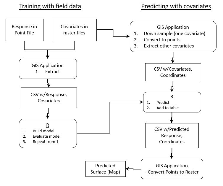
Below is a digram that summarizes this process: